Synthetic-Control Formalism
Let be the outcome for unit and period . Let denote treated units, eligible donors, and the last pre-treatment period after any window resolution.
For one treated unit, a synthetic counterfactual has the form
The maintained retrospective fast estimator uses pre-treatment features and post-period control outcomes to learn the match space. It does not fit to the treated post-period outcomes. The period effect is
and GeoSC’s top-level unscaled ATT is the average of that effect over measured post periods:
Read the fitted counterfactual
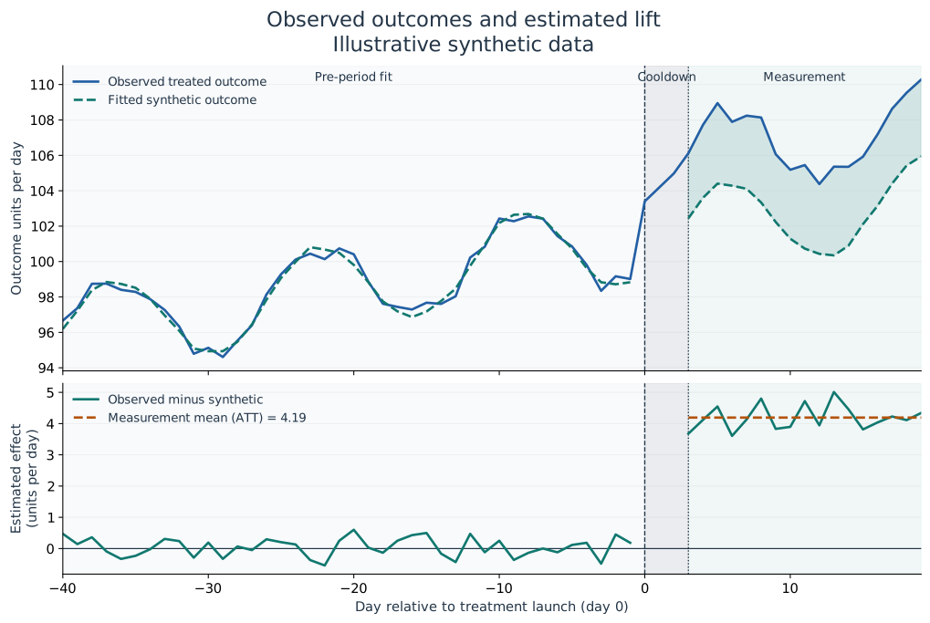
This illustrative synthetic example has one treated geography, 49 eligible controls, 40 pre-period days, three cooldown days and 17 measured days. The upper panel compares observed outcomes with the fitted synthetic trajectory. The lower panel shows their difference; its dashed line averages only measured days. The three cooldown days are excluded from fitting and the reported effect, so the synthetic line has a gap there. The filled area between the upper lines shows an outcome difference, not a confidence interval.
The generator adds four outcome units per day after launch, but the chart shows the estimated effect rather than substituting that known injection. Its counterfactual and placebo figures come from the same native GeoSC analysis. See the numerical source and reproduction instructions. This is an explanation of the calculation, not a calibration study or campaign result.
The implementation also supports multiple treated units. SparseSC constructs a joint treated effect and an in-space placebo reference set formed from treated- sized subsets of controls. With controls and treated units, the exhaustive assignment count is
GeoSC’s top-level p-value is not a post/pre mean-squared prediction-error ratio. If is the average placebo effect for assignment , SparseSC uses the two-sided absolute-effect comparison with add-one correction:
where is the effective exhaustive or sampled placebo count. The finest attainable step under this calculation is . The result is an empirical comparison against the eligible placebo assignments; its causal meaning depends on the design.